Learn how to display incoming audio data as a spectrum analyser by using the FFT class of the DSP module. Understand the benefits of using a windowing function.
Intermediate
Windows, macOS, Linux
dsp::FFT, dsp::WindowingFunction, Decibels
Getting started
This tutorial leads on from Tutorial: The fast Fourier transform. If you haven't done so already, you should read that tutorial first.
Download the demo project for this tutorial here: PIP | ZIP. Unzip the project and open the first header file in the Projucer.
- Note
- If your operating system requires you to request permission to access the microphone (currently iOS, Android and macOS Mojave) then you will need to set the corresponding option under the relevant exporter in the Projucer and resave the project.
If you need help with this step, see Tutorial: Projucer Part 1: Getting started with the Projucer.
The demo project
When completed, the demo project will display the incoming audio data as a two-dimensional spectrum analyser in the frequency (x-axis) and amplitude (y-axis) domains. The values displayed on the screen will be updated 30 times a second and the window at any time frame may look something like this:
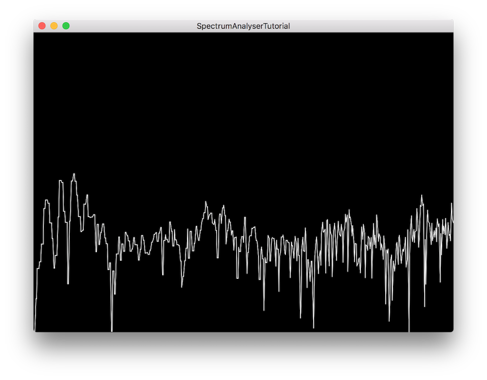
The demo project window
Windowing functions
As seen in Tutorial: The fast Fourier transform the Fast Fourier Transform allows us to convert a time domain signal to the frequency domain in order to process the individual frequency components of a certain signal.
However a limitation of the Fourier transform is that when applied during finite time intervals such as in audio buffer blocks of audio applications, the transformation manifests what we call spectral leakage where new frequency components start to appear on each side of the frequency in question. This is due to the fact that the sampled portion of the signal may not land on a natural period of the waveform which essentially truncates the signal.
Spectral leakage is especially problematic when analysing two sine waves with similar frequencies and similar amplitudes as well as two sine waves with dissimilar frequencies and dissimilar amplitudes. When the sine waves have close frequencies and amplitudes, leakage can render them indistinguishable from eachother. On the other hand, if the sine waves have far frequencies and amplitudes, leakage from the strongest component can mask the existence of the weakest.
To reduce the effect of spectral leakage, we can apply a windowing function to the signal before performing the Fourier transform and depending on the type of windowing, the effect on the output will be different. Here are some of the windows available in the JUCE DSP module and their characteristics:
- Rectangular: Lowest dynamic range, highest resolution. Equivalent to no windowing.
- Hamming: Fair dynamic range, good resolution. Typically used in narrow-band applications.
- Hann: Good dynamic range, fair resolution. Typically used in narrow-band applications.
- Blackman: Highest dynamic range, lowest resolution. Typically used in wide-band applications.
Processing Audio Data
Currently our application does not display nor process any incoming audio signals so let's start by implementing the FFT.
FFT Initialisation
In the AnalyserComponent class, start by declaring an enum as a public member to define useful constants for the FFT implementation:
enum
{
fftOrder = 11,
fftSize = 1 << fftOrder,
scopeSize = 512
};
- : The FFT order designates the size of the FFT window and the number of points on which it will operate corresponds to 2 to the power of the order. In this case, let's use an order of 11 which will produce an FFT with 2 ^ 11 = 2048 points.
- : To calculate the corresponding FFT size, we use the left bit shift operator which produces 2048 as binary number 100000000000.
- : We also set the number of points in the visual representation of the spectrum as a scope size of 512.
Next, declare private member variables required for the FFT implementation as shown below:
private:
juce::dsp::FFT forwardFFT;
juce::dsp::WindowingFunction<float>
window;
float fifo [fftSize];
float fftData [2 * fftSize];
int fifoIndex = 0;
bool nextFFTBlockReady = false;
float scopeData [scopeSize];
};
- : Declare a dsp::FFT object to perform the forward FFT on.
- : Also declare a dsp::WindowingFunction object to apply the windowing function on the signal.
- : The fifo float array of size 2048 will contain our incoming audio data in samples.
- : The fftData float array of size 4096 will contain the results of our FFT calculations.
- : This temporary index keeps count of the amount of samples in the fifo.
- : This temporary boolean tells us whether the next FFT block is ready to be rendered.
- : The scopeData float array of size 512 will contain the points to display on the screen.
Now let's initialise these variables in the member initialisation list of our constructor like so:
AnalyserComponent()
: forwardFFT (fftOrder),
{
The FFT object has to be explicitly initialised with the correct order at this point and the windowing function can be selected. In this case, we decide to use the Hann function but feel free to choose a different one.
In the overriden getNextAudioBlock() function, we simply push all the samples contained in our current audio buffer block to the fifo to be processed at a later time:
void getNextAudioBlock (const juce::AudioSourceChannelInfo& bufferToFill) override
{
if (bufferToFill.buffer->getNumChannels() > 0)
{
auto* channelData = bufferToFill.buffer->getReadPointer (0, bufferToFill.startSample);
for (auto i = 0; i < bufferToFill.numSamples; ++i)
pushNextSampleIntoFifo (channelData[i]);
}
}
To push the sample into the fifo, implement the pushNextSampleIntoFifo() function as described below:
void pushNextSampleIntoFifo (float sample) noexcept
{
if (fifoIndex == fftSize)
{
if (! nextFFTBlockReady)
{
juce::zeromem (fftData, sizeof (fftData));
memcpy (fftData, fifo, sizeof (fifo));
nextFFTBlockReady = true;
}
fifoIndex = 0;
}
fifo[fifoIndex++] = sample;
}
- : If the fifo contains enough data in this case 2048 samples, we are ready to copy the data to the fftData array for it to be processed by the FFT. We also set a flag to say that the next frame should now be rendered and always reset the index to 0 to start filling the fifo again.
- : Every time this function gets called, a sample is stored in the fifo and the index is incremented.
The fifo data now occupies the first half of the FFT input array and is ready to be processed and displayed.
Displaying the analyser
In the drawNextFrameOfSpectrum() function, insert the frame drawing implementation as explained below:
void drawNextFrameOfSpectrum()
{
window.multiplyWithWindowingTable (fftData, fftSize);
forwardFFT.performFrequencyOnlyForwardTransform (fftData);
auto mindB = -100.0f;
auto maxdB = 0.0f;
for (int i = 0; i < scopeSize; ++i)
{
auto skewedProportionX = 1.0f - std::exp (std::log (1.0f - (float) i / (float) scopeSize) * 0.2f);
auto fftDataIndex = juce::jlimit (0, fftSize / 2, (int) (skewedProportionX * (float) fftSize * 0.5f));
auto level = juce::jmap (juce::jlimit (mindB, maxdB, juce::Decibels::gainToDecibels (fftData[fftDataIndex])
- juce::Decibels::gainToDecibels ((float) fftSize)),
mindB, maxdB, 0.0f, 1.0f);
scopeData[i] = level;
}
}
- : First, apply the windowing function to the incoming data by calling the
multiplyWithWindowingTable() function on the window object and passing the data as an argument.
- : Then, render the FFT data using the
performFrequencyOnlyForwardTransform() function on the FFT object with the fftData array as an argument.
- : Now in the for loop for every point in the scope width, calculate the level proportionally to the desired minimum and maximum decibels. To do this, we first need to skew the x-axis to use a logarithmic scale to better represent our frequencies. We can then feed this scaling factor to retrieve the correct array index and use the amplitude value to map it to a range between 0.0 .. 1.0.
- : Finally set the appropriate point with the correct amplitude to prepare the drawing process.
Update the analyser using the timer callback function by calling the drawNextFrameOfSpectrum() only when the next FFT block is ready, reset the flag and update the GUI using the repaint() function:
void timerCallback() override
{
if (nextFFTBlockReady)
{
drawNextFrameOfSpectrum();
nextFFTBlockReady = false;
repaint();
}
}
As a final step, the paint() callback will call our helper function drawFrame() whenever a repaint() request has been initiated and the frame can be drawn as follows:
void drawFrame (juce::Graphics& g)
{
for (int i = 1; i < scopeSize; ++i)
{
auto width = getLocalBounds().getWidth();
auto height = getLocalBounds().getHeight();
g.drawLine ({ (float) juce::jmap (i - 1, 0, scopeSize - 1, 0, width),
juce::jmap (scopeData[i - 1], 0.0f, 1.0f, (float) height, 0.0f),
(float) juce::jmap (i, 0, scopeSize - 1, 0, width),
juce::jmap (scopeData[i], 0.0f, 1.0f, (float) height, 0.0f) });
}
}
Here, for every point in the array minus the first, we draw a line between the previous point and the current one by mapping the size of the scope to the size of the screen bounds.
- Exercise
- Try to change the windowing function used by the FFT and notice how differently the spectrum analyser reacts.
- Note
- The source code for this modified version of the code can be found in the
SpectrumAnalyserTutorial_02.h file of the demo project.
Summary
In this tutorial, we have learnt how to use a windowing function and an FFT to display audio data in a spectrum analyser. In particular, we have:
- Learnt the basics of a windowing function.
- Processed audio sample by sample using a fifo.
- Displayed the data by drawing lines between sample points.
See also
